Slow Manifold Gallery / Flow Manifold Gallery
Singularly Perturbed Systems
2D & 3D
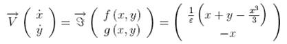
MF 30 Van der Pol model
![]()
Flow
Curvature Method, i.e., the 1st flow curvature
manifold directly provides the slow
invariant manifold associated with Van der Pol model.
1st
flow curvature manifold
singular
approximation
[1926]
Van der Pol, B., “On
’Relaxation-Oscillations’,” Phil. Mag., 7, Vol. 2.
MF 48 FitzHugh-Nagumo
model
The FitzHugh-Nagumo model (FitzHugh, 1961 ; Nagumo et al., 1962)
is a simplified version of the Hodgkin-Huxley model which models in a detailed
manner
activation and deactivation
dynamics of a spiking neuron. In the original papers of FitzHugh
this model was called “Bonhoeffer-Van der Pol oscillator”, since it
contains the van der
Pol oscillator as a special case for a = b = 0.
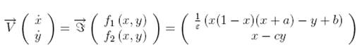
x denotes the
membrane potential, y is a recovery variable and b is the
magnitude of stimulus current
![]()
Flow
Curvature Method, i.e., the 1st flow
curvature manifold directly provides the slow invariant manifold associated with FitzHugh-Nagumo
model.
1st
flow curvature manifold
singular
approximation
[1961]
FitzHugh, R., “Impulses and physiological states in
theoretical models of nerve membranes,” 1182-Biophys. J., 1, 445-466.
[1962] Nagumo J. S., Arimoto S. & Oshizawa S., “An active pulse transmission line simulating
nerve axon,” Proc. Inst. Radio Engineers. 50, 2061-2070.
MF49 cubic Chua’s model
The cubic Chua’s
circuit (Chua et al., 1986) is an electronic circuit comprising an
inductance L1, an active resistor R, two capacitors C1 and
C2, and a nonlinear
resistor. Chua’s circuit
can be accurately modeled by means of a system of
three coupled first-order ordinary differential equations in the variables x
(t), y (t) and
z (t), which
give the voltages in the capacitors C1 and C2, and the intensity
of the electrical current in the inductance L1, respectively.
The function k(x)
describes the electrical response of the nonlinear resistor, i.e., its
characteristics which is a “cubic” function is defined by:
![]()
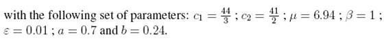
where the real
parameters c1 and c2 are determined by the particular values of
the circuit components.
Flow
Curvature Method, i.e., the 2nd flow
curvature manifold directly provides the slow invariant manifold associated with cubic Chua’s model.
[1986] Chua, L. O., Komuro,
M. & Matsumoto, T., “The double scroll family,” IEEE Trans. on Circuits and
Systems, 33, Vol.11, 1072-1097.
Non-singularly Perturbed
Systems 2D & 3D
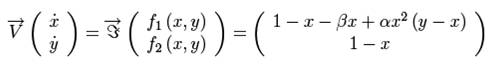
MF 50 Brusselator model
Studying an hypothetical chemical reaction in which it is assumed
that the reactions are all irreversible a
![]()
According to Grasman (1987) the chemical oscillation turns into relaxation oscillations. Thus, the Brusselator may be considered as slow-fast dynamical
systems although it has no small multiplicative parameter in its velocity
vector field and so no singular approximation.
Although the Brusselator model is not singularly
perturbed it can be considered as a slow fast dynamical system since
it may be shown (numerically) that its functional Jacobian
matrix exhibits a fast eigenvalue.
Flow
Curvature Method, i.e., the 1st flow
curvature manifold directly provides the slow invariant manifold associated with Brusselator
model.
[1967]
Prigogine, I. & Lefever, R. “On Symmetry-Breaking
Instabilities in Dissipative Systems,” Journal of Chemical Physics, Vol. 46,
3542-3550.
[1987]
Grasman, J., Asymptotic Methods for Relaxation
Oscillations and Applications, vol. 63,
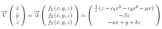
MF 50 Lorenz model
In the beginning of
the sixties a young meteorologist of the M.I.T., Edward N. Lorenz, was working
on weather prediction. He elaborated a model derived from
the Navier-Stokes equations with the Boussinesq
approximation, which described the atmospheric convection. Although his model
lost the correspondence to the actual atmosphere in the process of
approximation, chaos appeared from the equation describing the dynamics of the
nature. Let’s consider the Lorenz model (Lorenz, 1963):
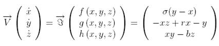
![]()
Although the Lorenz model is not singularly perturbed it can be
considered as a slow fast dynamical system
since it may be shown (numerically)
that its functional Jacobian matrix exhibits a fast
eigenvalue.
Flow
Curvature Method, i.e., the 2nd flow
curvature manifold directly provides the slow invariant manifold associated with Lorenz model.
[1963] Lorenz, E. N., “Deterministic non-periodic flows,” J. Atmos. Sc, 20,
130-141.
MF 51 Pikovskii-Rabinovich-Trakhtengerts model
The Pikovskii-Rabinovich-Trakhtengerts model (PRT) (Pikovskii et al., 1978) has been elaborated in order
to study interactions between “whistler waves” which propagate parallel to the
magnetic field and lower hybrid waves in a plasma. Such interactions are among
the important phenomena taking place in the ionosphere. This phenomenon can be modeled by means of a system of three coupled first-order
ordinary differential equations in the variables x(t), y(t)
and z(t), which give the the normal
amplitude of the wave, the normal amplitude of the ion acoustic wave and the
normal amplitude of the synchronous third wave produced, respectively. The
amplitudes are assumed to be constant in space. The evolution equations of the
(PRT) model may be written in dimensionless form:
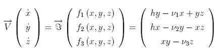
where the amplitudes
have been nondimensionalized; h is proportional
to the amplitude of the electric field of the “whistler” and v1 and v2
are the damping decrements of the excited hybrid and acoustic waves normalized
to the damping of the decay-induced third wave.
It has been
recently established (Llibre et al., 2008)
that this dynamical system exhibits a four wings butterfly chaotic attractor
for a particular set of parameters.
Although the (PRT) model is not singularly perturbed it can be
considered as a slow fast dynamical system
since it may be shown (numerically)
that its functional Jacobian matrix exhibits a fast
eigenvalue.
Flow
Curvature Method, i.e., the 2nd flow
curvature manifold directly provides the slow invariant manifold associated with (PRT) model.
[1978]
Pikovskii, A. S., Rabinovich,
M. I. & Takhtengerts, V. Y., “Onset of stochasticity in decay confinement of parametric
instability,” Soc. Phys. J. E. T. P., t. 47, 715-719.
[2008]
Llibre, J., Messias, M.
& Silva, P. R., “On the global dynamics of the Rabinovich
system,” J. Phys. A: Math. Theor. 41, 275210.
Singularly Perturbed Systems
4D & 5D
MF 55 fourth-order cubic Chua’s model
The fourth-order
cubic Chua’s circuit (Thamilmaran et al.,
2004, Liu et al., 2007) may be described starting from the same set of
differential equations as previously but while replacing the piecewise linear
function by a smooth cubic nonlinear.
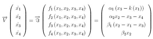
The function k (x1)
describing the electrical response of the nonlinear resistor is an
odd-symmetric function similar to the piecewise linear nonlinearity k (x1)
for which the parameters c1 = 0.3937 and c2 = -0.7235
are determined while using least-square method (Tsuneda,
2005) and which characteristics is defined by:
![]()
![]()
![]()
Flow
Curvature Method, i.e., the 3rd flow
curvature manifold directly provides the slow invariant manifold associated with cubic Chua’s model.
[2004]
Thamilmaran, K., Lakshmanan
M. & Venkatesan A. “Hyperchaos
in. a modified canonical Chua’s circuit,” Int. J. Bifurcation and Chaos,
vol. 14, 221-243.
[2007]
Liu X., Wang, J. & Huang, L., “Attractors of Fourth-Order Chua’s Circuit
and Chaos Control,” Int. J. Bifurcation and Chaos 8, Vol. 17, 2705
-2722.
MF 56 fifth-order cubic Chua’s model
The fifth-order
cubic Chua’s circuit (Hao et al., 2005) may be
described starting from the same set of differential equations as previously but
while replacing the
piecewise linear function by a smooth
cubic nonlinear.
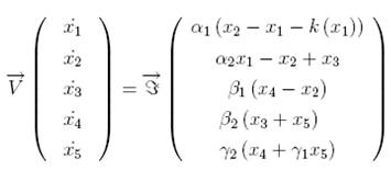
The function k (x1)
describing the electrical response of the nonlinear resistor is an
odd-symmetric function similar to the piecewise linear nonlinearity k (x1)
for which the parameters c1 = 0.1068 and c2 = -0.3056
are determined while using least-square method (Tsuneda,
2005) and which characteristics is defined by:
![]()
![]()
![]()
![]()
Flow
Curvature Method, i.e., the 4th flow
curvature manifold directly provides the slow invariant manifold associated with cubic Chua’s model.
[2005] Hao, L., Liu, J. & Wang, R., “Analysis of a Fifth-Order
Hyperchaotic Circuit,” in IEEE Int. Workshop VLSI
Design & Video Tech., 268-271.
[2005]
Tsuneda, A., “A gallery of attractors from smooth
Chua’s equation,” Int. J. Bifurcation and Chaos, vol. 15, 1- 49.
Non-singularly Perturbed
Systems 4D & 5D
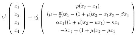
MF 57 Homopolar dynamo model
Homopolar dynamo model are used
for the understanding of spontaneous magnetic field generation in magnetohydrodynamics. In the seventies H. K. Mofatt (1978) proposed a model of coupled Faraday-disk homopolar dynamos. By introducing fluxes variables instead
of the currents this model has been transformed (Hide et al., 1999) into
the following dimensionless one:
![]()
Although the homopolar dynamo model is not singularly perturbed it
can be considered as a slow fast dynamical system since it may be shown
(numerically) that its functional Jacobian matrix
exhibits a fast eigenvalue.
Flow Curvature Method, i.e., the 3rd flow curvature manifold
directly provides the slow invariant
manifold associated with Mofatt model.
[1978]
Mofatt, H. K., Magnetic field generation in electrically
conducting fluids, Monograph in CUP series on Mechanics and Applied
Mathematics. (Translated from Russian).
[1999] Hide, R.
& Moroz,
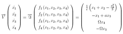
MF 58 Magnetoconvection model
A fifth-order
system for magnetoconvection (Knobloch
et al., 1981) is designed to describe nonlinear coupling between
Rayleigh-Bernard convection and an external magnetic field. This type of system
was first presented by Veronis (Veronis,
1966) in studying a rotating fluid. The fifth-order system of magnetoconvection is a straightforward extension of the
Lorenz model for the Boussinesq convection
interacting with the magnetic field. The fifth-order autonomous system of magnetoconvection is given as follows:
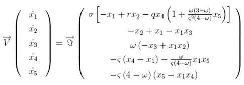
where x1(t)
represents the first-order velocity perturbation, while x2 (t), x3
(t), x4 (t) and x5 (t) are measures of the
first- and the second-order perturbations to
![]() the temperature and to
the magnetic flux function, respectively. With the five real parameters where is the magnetic Prandtl number (the ratio of the
the temperature and to
the magnetic flux function, respectively. With the five real parameters where is the magnetic Prandtl number (the ratio of the
![]() magnetic to the thermal
diffusivity), is the Prandtl
number, r = 14.47 is a normalized Rayleigh number, q
= 5 is a normalized Chandrasekhar number, and
magnetic to the thermal
diffusivity), is the Prandtl
number, r = 14.47 is a normalized Rayleigh number, q
= 5 is a normalized Chandrasekhar number, and
![]() is a
geometrical parameter
is a
geometrical parameter
Although the magnetoconvection model is not singularly perturbed it
can be considered as a slow fast dynamical system since it may be shown
(numerically) that its functional Jacobian matrix
exhibits a fast eigenvalue.
Flow Curvature Method, i.e., the 4th flow curvature manifold
directly provides the slow invariant
manifold associated with magnetoconvection model.
[1966]
Veronis, G., “Motions at subcritical values of the
Rayleigh number in a rotating fluid,” J. Fluid Mech., Vol. 24, 545–554.
[1981]
Knobloch, E. & Proctor, M., “Nonlinear periodic
convection in double-diffusive systems,” J. Fluid Mech. 108, 291-316.
Non-Autonomous Dynamical
Systems
MF 60 Forced Van der Pol model
In order to
highlight the efficiency of the Flow
Curvature Method, i.e., that it may extended to non-autonomous dynamical
systems let’s consider the forced Van der Pol model (Guckenheimer et al., 2002)
which may be written as:
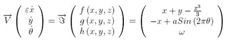
A variable changes may transform this non-automous
system into an autonomous one which reads:
![]()
Although this
transformation increases the dimension of the system the
Flow Curvature Method enables
to directly compute the slow manifold analytical equation associated
with system.
Flow Curvature Method, i.e., the 3rd flow curvature manifold
directly provides the slow invariant
manifold associated with Forced Van der Pol model.
[2002] Guckenheimer, J., Hoffman, K. & Weckesser,
W., “The forced van der Pol
equation I: the slow flow and its bifurcations,” SIAM J. App. Dyn. Sys., 2, 1-35.